How much autoregressive training does Diffusion Language Model need?
A small-scale experiment on whether diffusion language models should really be initialized from almost-fully-trained autoregressive checkpoints.
Table of Contents
As mentioned in the previous post, I will cover in this post my term project for Sewon’s class, where I studied a simple curriculum for pretraining block-diffusion language models. (Full report PDF · codebase)
Motivation
Diffusion language models (dLMs) are expensive to pretrain: any-order denoising is a strictly harder objective than left-to-right next-token prediction, and it costs more per training token. Faced with that cost, the field has split into two camps — and you can describe both with a single number, \(p_{\mathrm{AR}}\), the fraction of the total training budget spent on the AR objective.
Camp 1: convert an AR model (\(p_{\mathrm{AR}} \approx 1\)). Essentially every recent at-scale dLM is built this way: take a strong pretrained AR checkpoint, then run a comparatively brief diffusion-adaptation phase.
| Model | Recipe | Effective source fraction |
|---|---|---|
| Dream-7B | Qwen2.5-7B (~18T tokens) + 580B diffusion tokens | \(p_{\mathrm{AR}} \approx 0.97\) |
| DiffuLLaMA | LLaMA-2 (~2T) + ~65B adaptation tokens | \(p_{\mathrm{AR}} \approx 0.97\) |
| SDAR | Qwen3 (~36T) + 50B adaptation tokens | \(p_{\mathrm{AR}} \approx 0.999\) |
| LLaDA-2 | 3-phase block-WSD adaptation from an AR base | \(p_{\mathrm{AR}} \approx 1\) |
The implicit hypothesis here is “train autoregressively as long as possible, then briefly adapt.” It is justified by the observation that small-block diffusion is itself nearly autoregressive, plus the practical fact that an AR base usually already exists. (BD3LM follows the same source-heavy convention with a diffusion source instead — 850K MDLM steps + 150K block-diffusion steps, \(p_{\mathrm{MDLM}} = 0.85\) — which my MDLM-init track tests directly.)
Camp 2: full diffusion from scratch (\(p_{\mathrm{AR}} = 0\)). The dLM-bullish position points to data efficiency: dLMs are claimed to be “super data learners” — when unique training data is limited, they keep improving past the point where AR overfits, and small dLMs can eventually match or surpass AR baselines on downstream tasks. On this view, AR pretraining is at best a detour: if diffusion is the better objective, why spend any compute teaching the model a left-to-right habit it doesn’t ultimately want?
Both camps sit at the endpoints of the same knob, and the middle of the \(p_{\mathrm{AR}}\) range is completely unexplored. So the question this project asks:
If we actually believed the final model should be a diffusion model, how much AR pretraining would we choose on purpose?
My answer, at the scale I could afford to test: neither extreme. In my sweep, spending about 30% of the budget on AR and then switching to small-block diffusion beat pure-from-scratch diffusion and the AR-heavy conversions, at every block size where the comparison makes sense. Camp 1 spends at least 2.5× too large a fraction of its budget on AR; Camp 2 leaves transferable AR skills on the table.
Architecture
Before the actual curriculum research, I used this opportunity to practice architecture research. I started from a LLaMA-style 70M transformer and layered in interventions from recent work: QK-norm, per-head attention gates, depth-scaled layernorm, value residuals, ReGLU, RMSNorm, and interleaved MoE layers. The optimizer is NorMuon + AdamW: Muon handles matrix parameters, AdamW handles embeddings, the tied LM head, and scalar parameters (Adam betas \((0.95, 0.99)\), 100-step warmup, then constant LR).
A side question I wanted to answer: most architecture papers study AR models — do the same tricks help once the objective changes to diffusion? My short answer: yes, and by almost the same margins. Best validation loss over matched 5,100-step runs, under both objectives (Δ = relative improvement over the plain baseline):
| Configuration | AR | Δ | MDLM | Δ |
|---|---|---|---|---|
| Plain transformer (RoPE, ReGLU, RMSNorm) | 2.8529 | — | 3.1770 | — |
| + attention bundle (QK-norm, value residuals, per-head gating, depth-scaled LN) | 2.7686 | +3.0% | 3.0843 | +2.9% |
| + MoE only | 2.8062 | +1.6% | 3.1525 | +0.8% |
| + MoE and attention bundle (used in all curriculum runs) | 2.7523 | +3.5% | 3.0771 | +3.1% |
The attention bundle transfers almost exactly (+3.0% AR vs. +2.9% MDLM), MoE alone helps less under diffusion (+1.6% vs. +0.8%), and the combination is the best configuration under both objectives. The MoE+bundle MDLM run also had the healthiest routing (tail dropped-token fraction 0.004% vs. 1.6% for plain MoE). This part wasn’t the headline result, but a curriculum experiment is only meaningful if the underlying model isn’t falling apart for unrelated reasons — and it’s where I learned to train MoE models, watch router health, and read what optimizer choices do to loss curves.
Method
Block diffusion (BD3) gives a clean way to frame the problem. AR is block size \(b = 1\): predict left to right. Full masked diffusion (MDLM) is block size \(b = L\): denoise the whole sequence at once. BD3 sits in between: decode blocks left to right, but do diffusion-style denoising within each block. So a two-stage curriculum is parameterized by \((p_{\mathrm{AR}}, b)\):
- Train autoregressively (block size 1) for the first \(p_{\mathrm{AR}}\) of the optimizer-step budget.
- Switch to BD3 with block length \(b\) for the rest.
Existing A2D conversion is exactly this curriculum with \(p_{\mathrm{AR}}\) pinned near 1, and scratch BD3 is \(p_{\mathrm{AR}} = 0\). I swept the middle: \(p_{\mathrm{AR}} \in \{0.30, 0.50, 0.80, 0.90, 0.95\}\) crossed with post-switch block lengths \(b \in \{4, 16, 64, 256\}\), at 70M MoE scale on ClimbMix (sequence length 512, batch 512, 10,100 optimizer steps ≈ 1.54B unique tokens). I also ran the MDLM-init analogue, where the source phase is full-sequence diffusion instead of AR.
Result 1: the optimum is at 30% AR
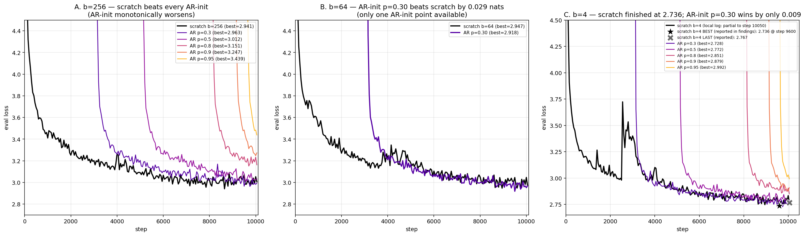
Best validation loss over the full run, AR-init grid (bold = best per column):
| \(p_{\mathrm{AR}}\) | \(b=4\) | \(b=64\) | \(b=256\) |
|---|---|---|---|
| 0.00 (scratch) | 2.7364 | 2.9467 | 2.9408 |
| 0.30 | 2.7275 | 2.9179 | 2.9629 |
| 0.50 | 2.7717 | — | 3.0124 |
| 0.80 | 2.8511 | — | 3.1512 |
| 0.90 | 2.8786 | — | 3.2469 |
| 0.95 | 2.9924 | — | 3.4385 |
Three things to notice. For every populated row, the best block length is \(b = 4\). For every column except \(b = 256\), the best switch point is \(p_{\mathrm{AR}} = 0.30\) — it beats scratch and beats every AR-heavy curriculum. And the AR-heavy corner where current practice lives (\(p_{\mathrm{AR}} \ge 0.8\)) is the worst part of the populated range, monotonically degrading as \(p_{\mathrm{AR}}\) grows.
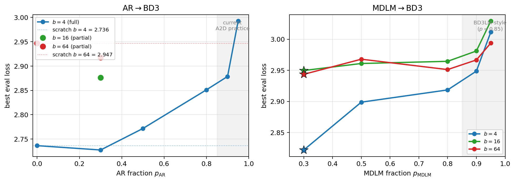
The MDLM-init track tells the same story: among MDLM→BD3 runs, \(p_{\mathrm{MDLM}} = 0.30\) wins at every \(b \le 64\), though it transfers less cleanly than AR-init does (at \(b = 4\) it loses to scratch by 1.6%). Interpolating my grid, BD3LM’s published recipe (\(p_{\mathrm{MDLM}} = 0.85\)) lands roughly 3.7% worse in validation loss than the \(0.30\) switch point at the same block size.
Result 2: the optimum doesn’t care about block size
The result that surprised me most isn’t that 30% is good — it’s that the same 30% is optimal at \(b = 4\), \(16\), and \(64\), in both curriculum families. Naively, I expected the optimum to slide with block size: \(b = 4\) is nearly autoregressive, so it should want lots of AR pretraining; \(b = 64\) is much less AR-like, so it should want less. (Strictly, since a larger \(b\) makes the post-switch task less AR-like, the optimum can only move downward with \(b\) — which is why I didn’t bother running \(p_{\mathrm{AR}} > 0.30\) at \(b = 64\).) Instead, the optimum didn’t move at all up to \(b = 64\).
The hypothesis: transferable AR skills are block-size-independent, and they saturate early
That bolded sentence is my hypothesis behind the project’s main result — it explains both results above, not just the invariance — so it deserves unpacking. Decompose what pretraining teaches into three buckets:
- Generic language skills: token statistics, vocabulary, syntax, semantics. Both objectives need these, AR learns them cheaply — and crucially, the AR phase is literally identical no matter which \(b\) you later switch to, so whatever it teaches that BD3 can reuse is shared across all block sizes. These skills saturate early, with strong diminishing returns.
- AR-specific machinery: mechanisms for predicting the next token from a left context alone. Past the early phase, this is mostly what additional AR training buys — and it need not transfer.
- Diffusion-specific machinery: mask-token handling, bidirectional reasoning within a block, denoising at varying mask rates. AR training never touches these; they converge slowly, and every extra AR step delays them.
Here’s a concrete toy example of why bucket 2 can be dead weight. Imagine training data containing strings like “\(A = p_1 \times p_2\)” where \(p_1 = 99{,}991\) and \(p_2 = 100{,}003\) are primes, so \(A = 9{,}999{,}399{,}973\). An AR model that sees “\(A =\)” and must predict the right-hand side has to learn integer factorization — a genuinely hard mechanism. A BD3 model that sees “\(A = \_ \times p_2\)” only needs to divide. The two objectives reward fundamentally different computations, and AR’s hard-won factorization circuit is useless under BD3 regardless of block size.
This decomposition turns the optimal switch point into a statement about marginal value: stay on AR while the next AR step’s transferable contribution (bucket 1) exceeds what a BD3 step at the same compute would buy (bucket 3), and switch the moment it drops below. Every piece of the main result falls out of this:
- The optimum is strictly positive. Bucket 1 is real, and AR learns it more cheaply than diffusion does — so scratch BD3 (\(p_{\mathrm{AR}} = 0\)) wastes expensive diffusion steps on skills AR would have taught faster. Hence 0.30 beats scratch.
- The optimum is far below 1. Bucket 1 saturates early; after that, AR compute buys mostly bucket 2 while bucket 3 sits untouched. Hence 0.30 beats 0.95, and Camp 1’s \(p_{\mathrm{AR}} \approx 0.97\) is deep in the dead-weight regime.
- The optimum is block-size invariant. Both the transferable bucket and its saturation curve are properties of the AR phase, which doesn’t depend on \(b\). Hence the same 0.30 at \(b = 4\), \(16\), and \(64\).
The hypothesis also predicts its own boundary: if \(b\) grows so large that the post-switch task is distributionally far from AR, even bucket 1 stops transferring, and the optimal \(p_{\mathrm{AR}}\) should collapse to zero.
The exception: half-sequence blocks
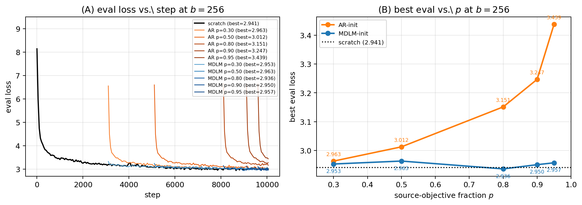
That is exactly what happens at \(b = 256\) (half the sequence length): the curriculum collapses, every AR-init run blows past scratch immediately after the switch and never recovers, monotonically worse in \(p_{\mathrm{AR}}\). Once the diffusion task is distributionally far enough from AR, the warm start stops being a warm start, and the question “when do AR’s marginal returns drop below BD3’s?” answers itself — immediately. Interestingly, MDLM-init partially survives at \(b = 256\) — MDLM features are themselves diffusion-flavored, so some transfer remains even at large blocks.
Data-limited regime
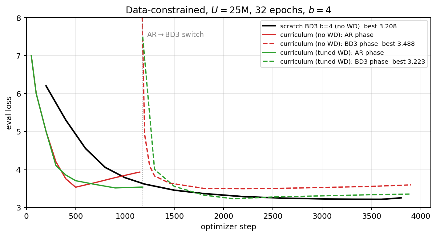
dLMs are often motivated by data efficiency: when unique data is limited and you train for many epochs, diffusion keeps improving after AR starts overfitting. So the regime that actually motivates dLMs is exactly the regime where an AR warm start sounds risky. I tested the curriculum at unique-data pools \(U \in \{25\mathrm{M}, 50\mathrm{M}\}\) tokens, 32 epochs each, \(b = 4\):
| Method | \(U = 25\mathrm{M}\) | \(U = 50\mathrm{M}\) |
|---|---|---|
| Scratch BD3 (no WD) | 3.2079 | 2.9509 |
| Curriculum, naive (\(p_{\mathrm{AR}}=0.30\), no WD) | 3.4884 | 3.1083 |
| Curriculum, tuned (\(p_{\mathrm{AR}}=0.30\), AR-phase WD) | 3.2231 | 2.9603 |
The naive recipe fails badly — 0.16 to 0.28 nats behind scratch. Inspecting the runs showed why: the AR phase overfits early (at \(U = 25\mathrm{M}\) its best eval comes at epoch 4, then degrades by ~0.4 nats before the handoff), and in parallel the MoE router collapses (final router entropy 0.747, 3% of tokens dropped). The BD3 continuation inherits a damaged router and never catches up.
The fix was phase-specific regularization: weight decay during the AR phase only (Muon WD 0.1 on matrices, small Adam WD, no router WD; all WD off during the BD3 phase). This flattens the AR phase, preserves the router (entropy 1.001, 0.04% dropped), and closes the gap to scratch from 0.28 to 0.015 nats at \(U = 25\mathrm{M}\).
One observation worth recording, with caution since it comes from a single pair of runs: at \(U = 50\mathrm{M}\), the tuned AR phase had worse AR validation loss than the unregularized one (3.290 vs. 3.246) but produced a BD3 continuation 0.148 nats better — in this pair, router health rather than AR loss predicted the quality of the continuation. It’s tempting to read this as “the best AR checkpoint is not the best initialization,” but MoE training is sensitive to hyperparameters, and some of these gaps may simply reflect configurations I didn’t tune hard enough.
The conclusion I’m more confident in is as follows, which I think is more interesting. I did not try hard here: a small, reasonable weight-decay grid on the AR phase alone was enough to bring the curriculum within 0.01–0.015 nats of scratch BD3. If scratch diffusion at 32 epochs is already close to the irreducible loss for these data pools — plausible, though I haven’t verified it — then matching it is the best any initialization could do. Read that way, the result is: even in the multi-epoch regime where AR famously overfits, spending 30% of the budget on AR pretraining (perhaps counterintuitively) does not harm the diffusion model you end up with.
Caveats
I don’t want to oversell a 70M-scale experiment, so the caveats up front. My budget is fixed in optimizer steps, not wall-clock: AR steps are roughly 5× cheaper than BD3 steps in my implementation, so a wall-clock-fixed comparison would favor a larger \(p_{\mathrm{AR}}\). Everything is validation loss — at this scale downstream benchmarks are noise. The optimum almost certainly depends on scale, sequence length, and architecture (though as a downward data point, a 1M-parameter sweep on TinyShakespeare found the same 0.30 optimum). And MoE adds hyperparameter sensitivity that could shift absolute numbers.
My current recipe: when pretraining a small-block diffusion LM from scratch, spend ~30% of the budget on AR, then switch to BD3. If the data is multi-epoch, regularize the AR phase and watch the router. The exact number 30% is not a law of nature — but “convert a 97%-finished AR model” is not one either.
What I take away
Beyond the result, this project made me more excited about pretraining science. I like the combination of theory-shaped questions and very concrete engineering: optimizer state at the objective handoff, router entropy, weight-decay groups, loss curves that suddenly tell you something is wrong. And I like the discipline of compressing a question that sounds too large for my resources into one I can actually run.
A few months ago I did not know how to train these models. Over this project I learned to train MoE transformers, use Muon, implement diffusion objectives, and debug a curriculum that failed for a non-obvious reason. That is exactly the learning loop I want more of.
Next up: μP and when is it guaranteed to be useful? I will explain a paper I presented in Jason Lee’s seminar class.
Full report: A Block-Size Curriculum for Diffusion Language Model Pretraining. Code: Chang-Han-Chen/sample-efficient-dlm.