MoE autoresearch
My first attempt at autoresearch and scaling laws (codebase)
Table of Contents
After the diffusion LM project, I felt like I should do something more fundamental and principled. The field has made tremendous progress on autoregressive GPTs — the architectures, the optimizers, the scaling methodology, the whole modern recipe — and working on the exotic frontier without having internalized that recipe felt like building on sand. It seems more reasonable to stand on the shoulders of giants first: get my foundations in LLM research as solid as possible, then carry them wherever I go next. So that’s what this project is: architecture research on a plain autoregressive MoE, followed by an attempt to validate the findings the way the frontier labs do (I think), namely with scaling laws.
Tl;dr I didn’t manage to get autoresearch to generate interesting ideas that actually work. With Karpathy’s program.md, Codex (5.5 xhigh) basically just swept a finer and finer grid of hyperparameters. I then iterated through a few versions of the program, eventually getting it to run literature search and propose research, but none of the ideas panned out in the end. This could well be a test-time-compute issue — I only let it work over one night max per variant. So in the end I did the idea-generation myself and asked Codex to implement techniques like XSA, gated attention, and so on. The one trick Codex found on its own that did work: under a fixed wall-clock budget, making the first two FFN layers dense helps, mostly because it trains faster. To see whether these interventions survive at scale, I wrote a second program for scaling-law experiments, asked Codex to implement and babysit the runs, and collected the results. Excitingly, the gains look real at ~10× the original scale and aren’t diminishing! Though of course we’d need to go well beyond the \(\sim 4\times 10^{19}\) FLOPs of our biggest run to be sure.
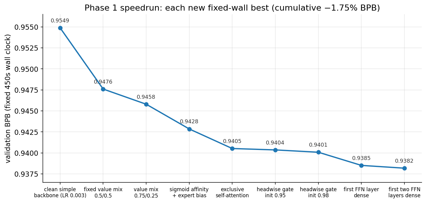
Here is the whole speedrun at a glance — every intervention that became the new fixed-wall best, stacking up to −1.75% BPB (how each works: Appendix A; how they were found: Phase 1):
A bunch of disclaimers upfront: our MoE router might be suboptimally tuned, though I put significant effort into making it at least look healthy; the scaling curve has fewer data points than I’d like; everything is single-seed; and there are no layer-specific hyperparameters like μP (so the embedding layer is likely undertrained), though I did sweep the global learning rate at each scale. I also did not do isoFLOP analysis to find compute-optimal ratio but assume Chinchilla ratio for active parameter count.
Still, I’m writing it up anyway. This is a learning process, and hopefully by exposing the process (mistakes included) I can collect some dense reward signals from the experts out there. Let me know if you have any feedback!
The project has two halves, and so does this post:
- A speedrun, in Karpathy’s autoresearch style. Starting from a deliberately stripped-down MoE transformer, Codex ran dozens of architecture experiments under a fixed 7.5-minute training budget on 4 H100 GPUs, following a protocol document I wrote. We kept five distinct interventions (eight leaderboard steps, since a few were bracketed in variants) — most of which came from me, though — improving validation bits-per-byte by 1.75%.
- A scaling check. We then ask the question that toy-scale architecture work usually dodges: do these wins survive when you scale the model up and train each size to a compute-optimal token budget, with paired controls?
Question: are architecture wins from a 7.5-minute speedrun real? Do they persist under compute-optimal scaling?
The answer, at the scale I could afford: mostly yes. The full intervention stack beats the simple backbone at 76M active parameters (by 1.49% relative BPB) and wins clearly at 185M (by 2.72%), but ties at 91M. So the gap is scale-positive but non-monotone. My hunch is that a good chunk of the gain comes from training stability: the baseline architecture showed repeated loss spikes and ended with visibly unhealthy routing even at 185M-active scale, while the recipe with our interventions stayed clean at every size up to 565M active parameters. A late ablation then rearranged my whole reading of the curve — it turns out most of the non-monotonicity traces to a single intervention (the dense stem), and removing it both flattens the gap and exposes the stability problem that motivates what I want to do next.
Phase 1: speedrun
Setup
Everything runs on Karpathy’s autoresearch, lightly adapted: a single train.py (the only file the agent may modify), a frozen prepare.py that downloads data and defines the benchmark, and two log files the agent must maintain. Data is ClimbMix, tokenized with a custom 8192-vocab BPE, sequence length 2048. Hardware is a 4×H100 node rented from VESSL AI and Vast.ai. As promised in my first post, this kind of research really is doable on a PhD student budget (but very tight😱).
The benchmark metric is validation bits-per-byte (BPB), following Karpathy: per-token cross-entropy summed over the bytes of the target text, rather than averaged over tokens. This makes models with different tokenizers comparable and prevents an architecture from “winning” by exploiting token granularity. Lower is better; at this scale, differences of ~0.001 BPB are meaningful and reproducible, which still surprises me.
The model family is a mixture-of-experts (MoE) transformer. Quick reminder on MoE: instead of every token passing through the same feed-forward network (FFN), each token is routed to a small subset of parallel FFNs (“experts”), so the model has far more total parameters than it spends compute on per token. In our case, each forward pass picks the top 2 of 16 experts, and the model has 438M total but only 91M active parameters. The catch is the router, a tiny linear layer that decides which experts see which tokens. It is notoriously hard to stably train the routers; a common instability is that a few experts happen to get routed more, get more gradient signals, perform better, and therefore get routed even more often. So, MoE experiments must track router health (load balance, entropy, per-expert load) alongside the loss. In my own experiments, many architecture interventions for dense transformers don’t work for MoE because they somehow mess up the router; for example, learnable value residual.
Each run trains for a fixed 450 seconds of measured wall-clock training time, then evaluates validation BPB. Fixed time, not fixed steps — so an intervention can win either by learning more per step or by simply being faster. This feels like a more practical setup, especially for MoE, where architecture choices (e.g. sparsity) often have a big impact on hardware efficiency (MFU, etc.).
My program.md
Karpathy’s original program.md didn’t work well for me — Codex mostly tweaked hyperparameters (which matters too! but I was hoping for more). So I reflected on my own research process, and the step that stood out was forming a hypothesis. There are always infinitely many ablations one could run, so the real skill is picking the ones that are most informative. Codex, left to itself, was often too hung up on being “rigorous” about uninformative ablations — grid-searching between two bad learning rates to “be absolutely sure we are not missing anything.” I wouldn’t do that, because I’d reason: “the loss should be locally convex in learning rate, and the curvature from the current grid says there’s no local optimum hiding between these points.” Once you have a falsifiable hypothesis like that, the next run either confirms it or kills it. I thought this was the missing ingredient, so I built it into my program.md.
Concretely, every run has to walk through this loop:
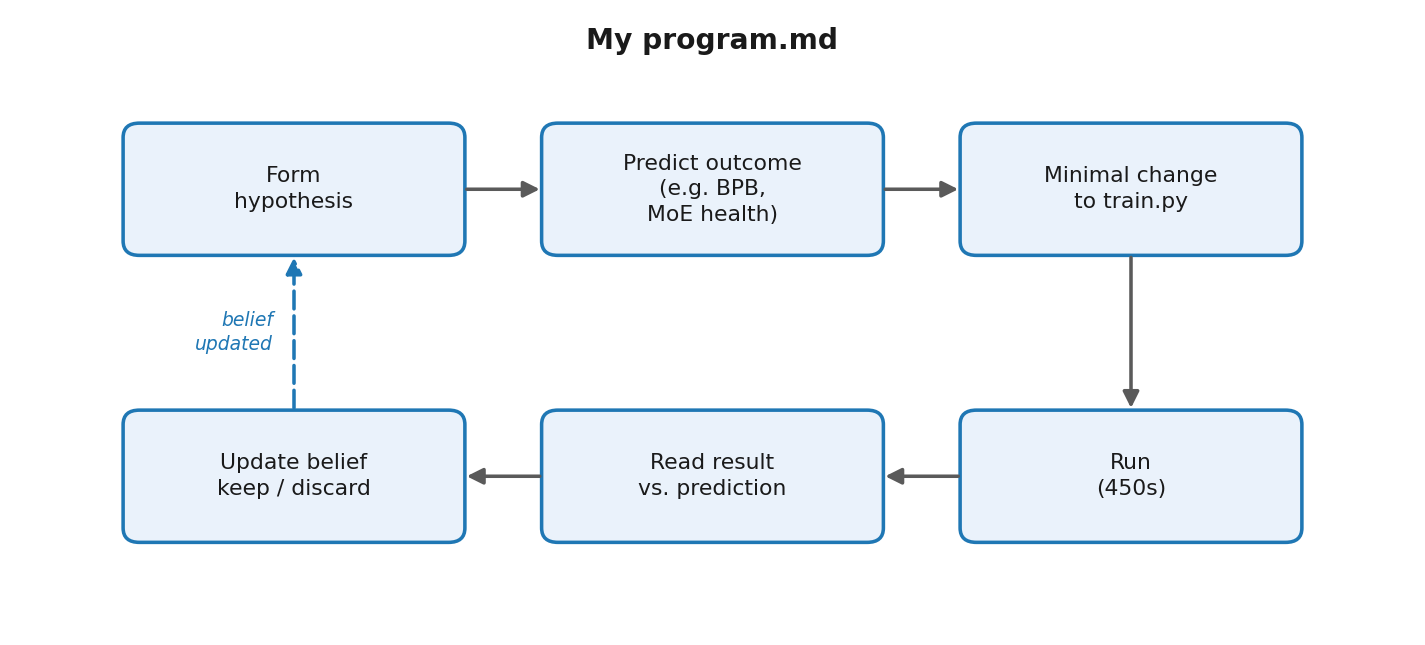
The key discipline is: write down the hypothesis before launching the run, then update the belief after reading the result. Do not blindly try changes; chase the highest signal.
Every run entry must contain a pre-run hypothesis, an expected result, the observed result, an interpretation, an explicit agrees with hypothesis: yes/no/partial, and a decision. Here’s a representative entry from the log, the one where exclusive self-attention got promoted to baseline:
Pre-run hypothesis: Exclusive self attention may improve the division of labor between attention and the MoE FFN by forcing attention outputs to carry contextual information orthogonal to the current token’s own value vector […]
Expected result: matched-step CE and final BPB should improve with minimal throughput cost. Router load should remain similar to the current best; if router diagnostics move sharply, the attention change is perturbing the sparse FFN rather than cleanly improving context modeling.
Observed result:
val_bpb 0.940518[…] validation improved by0.002330BPB. Router health remained acceptable: mean load CV0.094, max-layer max load0.122[…]Agrees with hypothesis: yes. Decision: keep as current best.
Note the expected result names a router diagnostic, not just BPB — so the run can fail in an interpretable way (a BPB gain bought with router damage would have been a discard, not a keep). As I write this, I realize what I’m really describing is something like active learning: pick the next experiment to maximize information gain. Maybe that’s the paradigm I’d advocate for AI scientists.
I also wanted the agent to find high-signal papers and reproduce them itself. Done naively, it overinvests in the first direction it likes. To force early exploration before committing, I set up a tournament-style search:
Run 20 search/reflection iterations, each scanning ~10 papers, selecting 2 one-sentence ideas with a written reason why those 2 beat the other 8, then updating the search keywords for the next iteration; afterwards, distill the 40 collected ideas through timed synthesis passes into a unified hypothesis and a ranked experiment queue, under a research filter the program calls “brutal: prefer ideas that can be stated in two sentences, implemented in a few lines, and tested with one clear diagnostic besides BPB.”
And I have to say, the output looks like research. A representative selection step from the literature log reads:
Selected: (1) MTP is a future-pressure regularizer: extra future heads force hidden states to encode constraints beyond the immediate next token. (2) TOP is a cheaper and possibly cleaner version of MTP: rank the true future tokens by closeness instead of asking the model to exactly classify every future token.
Why these two: They preserve the simple “future supervision” insight without requiring data labels or a new optimizer. TOP wins the first follow-up slot because it can be implemented by gathering logits for future targets and adding a small pairwise ranking loss.
The reading list it built is genuinely diverse and high-signal — selective token losses (Rho-1 style), multi-token and ranking objectives, JEPA-style latent targets, curriculum and data-ordering tricks — and the queue is sensibly prioritized by implementation cost. One idea I found genuinely novel: a byte-weighted cross-entropy, where each token’s loss is scaled by its byte length, on the reasoning that the eval metric (BPB) is measured per byte. I don’t think it’s especially well-motivated in the end — the standard per-token cross-entropy is already aligned with BPB up to a constant — and when we actually tried it, it didn’t help. But I’d never seen it before, and “invent a plausible-looking loss I haven’t seen” is at least a different failure mode from “tweak the learning rate.”
But when its ideas were actually implemented and tested, none of them earned a keep. My current guess is test-time compute: one night is enough to scan and rank a literature, but probably not enough to iterate on any single idea until the finicky details that make a paper’s trick work are faithfully reproduced. I’d honestly like to be wrong here, and I want to rerun this loop someday with a much bigger inference budget.
The program also hard-codes a couple of guardrails. The optimizer is frozen — Muon for matrices, AdamW for everything else — and only LR values may change. And the keep/discard rule has a router-health veto: any intervention that drives a layer into collapse (one expert taking ≥25% of top-2 traffic over 16 experts) cannot be kept, even if BPB improved — though in practice such runs underperformed anyway.
So in the end I generated the ideas myself, which is fine, since my priority here is learning. Of the five interventions in the final stack, I proposed four: the value residual (a damped value mix), DeepSeek’s aux-loss-free sigmoid router, exclusive self-attention, and the headwise attention gate (for taming attention sinks). The one original idea from Codex, not me, was making the first few FFN layers dense — though I later learned this is a common trick in open-source MoEs like DeepSeek-V3, which uses three dense layers; at our scale Codex found two was optimal.
Even so, I came away quite bullish on “AI doing AI research.” The execution and bookkeeping are already better than mine; what’s missing is the taste to pick the next question, and that may be more a matter of scaffold and inference budget than of raw capability. I suspect a richer scaffold — something with the evolutionary, population-based flavor of AlphaEvolve — would do meaningfully better.
The details follow.
The speedrun
The starting point is deliberately boring: an 8-layer, 768-dim transformer, 16 experts with top-2 routing and softmax token-choice, GQA + RoPE + QK-norm. From there, Codex worked through the intervention queue. Here is the full leaderboard — every run that became the new best (math and code for each in Appendix A); rather than narrate all ~30 runs, I’ll just tell the three stories I think teach the most.
| # | intervention | val BPB | Δ vs prev | cumulative |
|---|---|---|---|---|
| 0 | clean simple backbone, LR 0.003 | 0.954881 | — | — |
| 1 | fixed value mix \(0.5 v_1 + 0.5 v_\ell\) | 0.947597 | 0.763% | 0.763% |
| 2 | value mix \(0.75 v_1 + 0.25 v_\ell\) | 0.945791 | 0.191% | 0.952% |
| 3 | sigmoid affinities + expert bias + load-balance 0.003 | 0.942848 | 0.311% | 1.260% |
| 4 | exclusive self-attention | 0.940518 | 0.247% | 1.504% |
| 5 | headwise attention gate, init 0.95 | 0.940352 | 0.018% | 1.522% |
| 6 | headwise attention gate, init 0.98 | 0.940076 | 0.029% | 1.550% |
| 7 | first FFN layer dense | 0.938510 | 0.167% | 1.714% |
| 8 | first two FFN layers dense | 0.938179 | 0.035% | 1.749% |
Story 1: the value residual that failed, and the diagnostic that explained why
The first idea I queued was a ResFormer-style value residual: let later attention layers mix in the first layer’s value tensor through a learned scalar per layer, initialized at zero. In dense transformers this reliably helps. Here, it didn’t. Matched-step loss was no better and router load concentrated. The interesting part is what the agent did next. It ran a 120-second diagnostic on the gradients, then wrote what I consider the best paragraph in the entire log:
The scalar residual is not inert: mean absolute
value_resid_alphagrew from 0 to 0.225 by step 596, with one layer reaching 0.968. However, the residual path gradient into the retained first-layer value clone stayed tiny in absolute RMS […] The data argues against the “useful early value gradient highway” story for this exact form. The scalar learns a sizable residual mixture, but the visible effect is mostly representation/routing disturbance.
In other words: the mechanism story from the dense-model literature (“value residuals create a gradient highway to early layers”) measurably did not transfer. The learned mixture was changing the representations that later routers see, destabilizing expert load before delivering any gradient-flow benefit — a failure mode that simply cannot exist in a dense model, because dense models have no router to disturb. The repair, two runs later, was almost comically blunt: don’t learn the mixture at all. A fixed mix \(v = 0.75\,v_1 + 0.25\,v_\ell\) — first-heavy, damped, with nothing for the optimizer to over-adapt — turned the idea from harmful to a 0.95% cumulative win. Learned, normalized-learned, and larger-ratio variants were all tested; all lost. I would not have guessed that the difference between “harmful” and “best win of the phase” was removing the learnable parameter.
For full honesty, I did steer the agent a bit because I wanted to understand why value residual could work. So I asked it to monitor the gradient of mixing coefficient along with other things. I think somehow these observations that stayed in the chat history ended up inspiring the model to do the above. Nice collaboration, Codex.
Story 2: the router that collapsed on schedule, and the control that earned the win
The target was DeepSeek-V3-style routing (sigmoid affinities plus auxiliary-loss-free expert bias): score experts with independent sigmoids instead of a competitive softmax, and steer load not with a loss but with a non-gradient bias term that nudges selection toward underused experts.
Tested with zero load-balance loss — the purist version — it improved BPB, but the router looked unhealthy:
However, one layer collapsed: max-layer load CV 2.646, max-layer max load 0.500, min-layer router entropy 0.000884, and max router bias hit the 0.25 clamp.
One layer’s router sent half of all top-2 traffic to a single expert of sixteen. Here’s the part I’m proud of (as the program author): I saw this coming! I wrote in program.md that if loss-free balancing collapsed, the agent got exactly one run adding a small differentiable load-balance term, coefficient 0.003, no sweeping. That run fixed the collapse (max-layer max load 0.0746, basically uniform) and improved BPB further, to 0.942848.
If I were doing this alone, I would have declared victory already. But my rigorous partner, Codex, ran a control: same value mix, same small 0.003 coefficient, but with softmax routing. The control regressed badly to 0.947950 with terrible load (max-layer max load 0.485):
Lowering the load-balance coefficient is not sufficient. Without sigmoid/bias, softmax routing becomes highly imbalanced […] The best run’s improvement really depends on the sigmoid/bias router controller.
Without this control, the honest claim would have been “we changed two things and it got better.” With it, the mechanism is isolated. Doing such control ablations would have been mentally draining for me, so it is nice that AI can do it!
Story 3: Codex’s own idea
After the attention-side wins (exclusive self-attention, then a near-identity headwise sigmoid gate — see Appendix A; the gate-init bracketing 0.95 → 0.98 → 0.99 is a tidy little study in itself, converging on “as close to identity as possible but not closer”), the agent proposed the one original idea that survived: replace the first MoE FFN layers with plain dense SwiGLU layers of matched active width. The hypothesis, in its words,
early token representations may be “too raw for useful sparse routing,” so spend the first layers on a dense transformation and save the experts for later layers where routing decisions are better-informed.
One dense layer: 0.938510. Two dense layers: 0.938179, with total parameters down from 554M to 438M (each dense layer replaces a 16-expert bank) and throughput up (24.6% vs 22.3% MFU). Three dense layers: worse. The benefit saturates fast.
Ideas that failed
The log contains far more discarded runs than kept ones. Here are some of the most memorable ones.
I asked for depth-scaled residual scaling (multiply the layer-\(\ell\) branches by \(1/\sqrt{\ell}\), a trick with decent dense-model pedigree), and eight consecutive runs tried every placement: pre-norm, branch-only, MLP-only quarter-power (a cute hypothesis from Codex: SwiGLU is roughly quadratic in its input scale, so scale inputs by \(\ell^{-1/4}\) to get an \(\ell^{-1/2}\) branch), MLP+V, MLP+V+gate, V-only, V+gate, and finally output-side. Every variant lost. The ordering is at least informative — internal scaling was catastrophic, output-side merely bad — with a consistent moral: this model wants full-amplitude branches. The family was closed with the log’s dry “Close fixed deterministic layer scaling for now.” I forget whether we ever tried a learnable layer scale; I just remember being exhausted by that point.
Also in the pool: fine-grained experts (32 experts, top-4, half-width, preserving the active FFN width, total expert width, and sparsity ratio), which DeepSeek-style scaling folklore says should help. We tried it three times: once early, once re-tested on top of the stabilized router stack in case the old router had been the bottleneck, and once more in a dedicated fine-vs-coarse geometry check (0.953126 vs 0.935178, not close). Routing was perfectly healthy each time; the smaller experts just learned worse and dispatched slower at this scale and horizon. I file this under “folklore is scale-dependent” and would genuinely like to know where the crossover is.
Phase 2: scaling laws
This is the part of the project I was most excited about. Phase 2 got its own program, program_june_ninth.md, which is much more boring to read than the first one — and that’s by design. A scaling-law experiment is fairly standard: you specify the experiment design, then ask the model to babysit the runs while keeping an eye on MFU, throughput, loss spikes, and MoE health. The program defines five sizes, F1–F5 (depth 8→16, width 768→1792, 91M→852M active params), plus a smaller S75 anchor below F1. F5 ended up over my budget, so the curve runs S75 through F4. Each size trains to a compute-optimal token budget (~20 tokens per active parameter, the Chinchilla rule of thumb) with the learning rate re-swept on a coarse 3× grid, since — as I learned the hard way — the optimal LR drifts with scale.
Sweep sparsity again
I’d had a vague impression that in the compute-bound (i.e. effectively infinite data) regime, sparser is always better until you hit a memory wall. So I asked Codex to run the expert-count sweep one more time, this time on top of all the interventions. We fix the active expert count at top-2 and sweep the total expert count E ∈ {4, 8, 16, 32, 64, 128}:
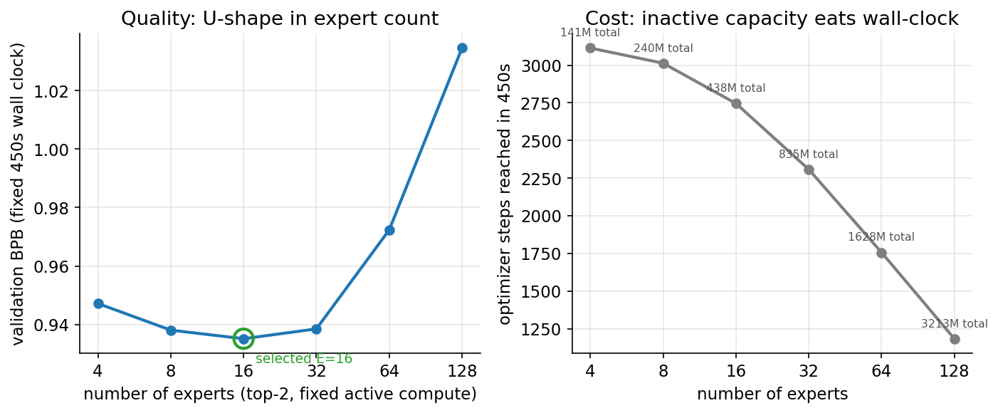
So maybe I was wrong: sparser is not always better, even with effectively infinite data. The BPB is U-shaped, bottoming out at E=16. In hindsight the intuition is simple — under a fixed wall clock, inactive parameters aren’t free (they cost optimizer state, memory traffic, and dispatch overhead), so the very sparse models train stably but get hopelessly outrun on tokens. Of course, this might also just be a skill issue in my router load-balancing… Either way, I picked E=16, top-2, 12.5% sparsity to scale.
Scaling result
| size | active params | tokens | full BPB | simple BPB | gap (rel.) |
|---|---|---|---|---|---|
| S75 | 76M | 1.5B | 0.902337 | 0.916017 | 1.49% |
| F1 | 91M | 1.8B | 0.892152 | 0.892165 | 0.00% (tie) |
| F2 | 185M | 3.7B | 0.821625 | 0.844628 | 2.72% |
| F3 | 352M | 7.0B | 0.765974 | — | — |
| F4 | 565M | 11.3B | 0.736565 | — | — |
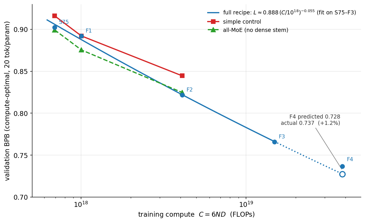
Since each size is trained roughly Chinchilla-optimally (~20 tokens per active parameter), I can put all five full-recipe points on a single compute axis, \(C = 6ND\) FLOPs (with \(N\) active params and \(D\) tokens), and ask whether they follow a scaling law. The usual form is a power law with an irreducible-loss offset,
\[L(C) = \frac{A}{C^{\alpha}} + B.\]Fitting this to the four smaller points (S75–F3) and holding out F4 turns out to be instructive: with only four points the offset \(B\) is badly under-determined — left unconstrained it runs to a nonsensical negative value, and the moment I bound it to be physical it collapses to \(B = 0\). In other words, over this ~20× span of fitted compute the data simply don’t yet bend enough to pin down a floor; they’re well described by a plain power law, \(L \approx 0.888\,(C/10^{18})^{-0.055}\). The exponent is tiny — loss falls slowly in compute, as it always does for language models — but the fit is clean (residuals under 0.005 BPB).
Extrapolating that fit out to F4’s compute (\(3.8\times10^{19}\) FLOPs, ~2.6× beyond the last fitted point) predicts BPB 0.728, while the actual F4 run came in at 0.737 — about 1.2% higher than the trend. So the held-out point lands close, but on the worse side: F4 slightly underperforms its own extrapolation. That’s the expected direction if F4 is a touch undertrained — recall its lower-LR arm was aborted before finishing — so I read this less as “the scaling law broke” and more as “I didn’t tune F4 as carefully as the smaller points.” Either way, a held-out point 2.6× beyond the fitted range landing within ~1% is more than I expected from five single-seed runs.
A few more observations:
The stack scales mechanically and stays healthy. Up to 565M active (3.3B total) parameters, there were no divergences, no router collapse, and near-uniform max-layer expert load at every size. That sounds like faint praise, but it isn’t: the simple control at F2 suffered repeated transient loss spikes above 6 during training and finished with a mean load CV of 0.52, against the full recipe’s 0.075. Part of what the intervention stack buys is apparently not lower loss but lower variance and router sanity at scale — which, at real scale, is worth more than the BPB itself, since a diverged run returns nothing.
The gap is scale-positive but non-monotone. At F1 the two recipes land within 0.000013 BPB of each other — a tie to four decimal places, at the exact configuration where the whole Phase 1 speedrun was run. This is a bit funny: the size where we did all the architecture search shows no compute-optimal-matched advantage at all, and the wins only separate at scales we never searched at. (Note that at fixed wall clock our recipe still wins even at F1, because it’s faster — the tie is specifically about quality at matched tokens.) It would have been nice to have baseline runs at F3 and F4 to make a more conclusive claim, but that’s beyond my current budget.
What about all-MoE at scale?
The two-dense stem is a crutch, and in the long run I’d like to drop it — once I’ve learned the modern tricks for stabilizing pure MoEs (Quantile Balancing, etc.), the early dense layers shouldn’t be necessary. So I ran the all-MoE ablation: the full intervention stack with the dense stem removed, every FFN layer sparse. The result was the most surprising of the project, and it’s what made me rewrite my reading of the whole curve.
At small scale, all-MoE wins: it beats the two-dense recipe by 0.0031 BPB at S75 and by a striking 0.0167 BPB at F1 (0.875 vs 0.892) — that’s the dashed green curve dipping below the blue one at the left of the figure. Recompute the gap against the simple control using all-MoE instead of the two-dense recipe, and the embarrassing non-monotonicity nearly vanishes: 1.83% at S75, 1.87% at F1, 2.36% at F2. In other words, the quality gain from the intervention bundle was consistent across scales all along; the F1 tie was the dense stem quietly giving that gain back. Under the fixed-wall speedrun, the stem’s throughput advantage hid this completely; under compute-optimal budgets, where speed buys nothing, the first two dense layers turn out to be a quality cost at small scale.
But — and this is why I can’t just delete the stem yet — the all-MoE F1 run finished with one router layer at max load 0.253, just over my 0.25 safety threshold, the only compute-optimal run in the whole project to cross it. And at F2 all-MoE flips to losing: 0.0031 BPB worse and meaningfully slower (23.5% vs 25.7% MFU, since every layer now pays dispatch overhead). The pattern across the three sizes is uncomfortable: at LR 0.003 the all-MoE model grows a hot layer as it scales; at F2’s gentler LR 0.001 it stays clean but can’t keep up. Either you flirt with instability or you pay a tax to avoid it. Seen this way, the dense stem was never really a quality intervention — it’s a stabilizer whose price grows with the compute budget, which is presumably why DeepSeek-V3 (trained at fixed token budgets, not fixed wall-clock) still ships dense early layers: at their scale, the insurance is worth it.
The model I actually want — fully sparse, no crutch, stable at every size — is sitting right there in the table, one imbalanced layer away. Hopefully I can remove the stem for real in the next iteration.
Final thoughts
Working with an AI agent on a research project was genuinely fun, and it made the whole learning experience much faster. For my own benefit, let me record where I land on “AI as an AI researcher” right now:
Great at: execution fidelity, log discipline, and negative-result hygiene. It never quietly dropped a failed run, always wrote down matched-step comparisons with exact numbers, aborted runs against criteria written down in advance instead of on hope, and once spent a whole diagnostic run instrumenting gradients to figure out why an idea failed rather than just recording that it did (this took some context engineering on my part; see Story 1). A surprising fraction of human research pathology is simply absent by default.
Bad at: knowing which question is worth asking next. Its failure mode isn’t laziness — it’s a kind of diligent myopia, generating an endless sequence of locally-justified next steps down whatever gradient is in front of it (finer LR grids, an eighth depth-scaling variant). And when I explicitly asked for creativity via the literature-search program, I got ideas that sounded interesting but didn’t land — plausibly for lack of iteration compute, as I keep saying.
Moving forward, my top priority is to stabilize MoE further, so I can finally remove those dense early layers. The scaling experiments convinced me that all-MoE wants to work and is just not stable enough yet. Quantile Balancing looks promising and is at the top of my list. The other thread is principled hyperparameter transfer — μP, or Complete(d)P.
But, well, I clearly set too high a goal again. The lesson of my PhD was to lower my standards (see my first post!), validate the simplest thing I can fully understand, and iterate — and this project is proof I still haven’t internalized it. “Stabilize all-MoE at every scale” is not the simplest thing I can fully understand; I can’t even claim to fully understand how to stabilize and scale a dense model yet. So, lower the standards once more: do μP on dense models first. That’ll hopefully be the next post. Then, with that foundation, back to MoE — implement QB, and work out how μP should behave for MoE.
Appendix
A: Intervention details
All code below is the actual train.py implementation (lightly trimmed). Notation: \(x \in \mathbb{R}^{B\times T\times d}\) is the residual stream, \(h\) heads, \(E=16\) experts, \(K=2\) active.
A.1 Fixed first-value mix
Idea. Layers \(\ell \geq 1\) compute attention not over their own value vectors \(v_\ell\) but over a fixed mixture with the first layer’s values:
\[v^{\text{mix}}_\ell = \alpha\, v_1 + \beta\, v_\ell, \qquad \alpha=0.75,\ \beta=0.25.\]This descends from value-residual learning (ResFormer): early value streams carry token-local information that later layers benefit from re-accessing directly. The MoE-specific twist, learned the hard way (Story 1), is that the coefficients must be fixed, first-heavy, and damped: a learned scalar version measurably disturbed the representations seen by downstream routers and concentrated expert load before delivering any benefit. Removing the learnable degrees of freedom is what made the idea work. Note \(\alpha+\beta=1\), so the mixed value’s scale stays comparable to a plain value vector.
# CausalSelfAttention.forward — v is this layer's values, first_v is layer 0's
layer_v = v   # cached so layer 0 can hand its values to later layers
if self.value_mix_enabled and first_v is not None:
    mixed_v = (self.value_mix_first.to(v.dtype) * first_v.to(v.dtype)
               + self.value_mix_local.to(v.dtype) * v)
    v = mixed_v
A.2 Sigmoid-affinity router with loss-free expert bias
Idea (from DeepSeek-V3 / aux-loss-free balancing). Two coupled changes to top-k token-choice routing.
Scoring. Replace softmax routing probabilities with independent sigmoid affinities. With router logits \(z = W_r x \in \mathbb{R}^E\):
\[a_i = \sigma(z_i), \qquad \text{output weight } w_i = \frac{a_i}{\sum_{j \in \text{top-}k} a_j} \ \text{ over selected experts only.}\]Softmax makes experts compete globally — pushing up one expert’s score necessarily pushes down the others’ — and this competition is entangled with the load-balancing gradients. Sigmoid scores each expert independently and normalizes only at the end, over the selected experts.
Load control. Instead of relying on an auxiliary loss, keep a non-gradient per-expert bias \(b\), updated from an EMA of realized hard load: experts above uniform load get pushed down, below get pushed up. Crucially, the bias affects selection only — output weights use the clean affinities, so the correction never contaminates the forward computation:
\[\text{select top-}k \text{ of } (a + b), \qquad \text{mix with } w(a) \text{ only}.\] \[b \leftarrow \mathrm{clamp}\!\left(b + \eta\, \frac{u - \mathrm{EMA}(\text{load})}{u},\ \pm 0.25\right), \qquad u = 1/E.\]The empirical footnote that matters: pure loss-free balancing collapsed one layer at this scale (Story 2). The working configuration keeps a small differentiable load-balance term, coefficient 0.003 — about 3× lighter than the softmax baseline needed — and the softmax control proved the mechanism is the sigmoid/bias controller, not the lighter coefficient.
# TokenChoiceMoE.forward — router math kept in fp32 under bf16 autocast
router_logits = self.router(flat_x.float())              # [N, E]
affinity = torch.sigmoid(router_logits)
route_scores = affinity + self.router_bias                # bias: selection only
_, top_idx = torch.topk(route_scores, K, dim=-1)
clean_scores = affinity.gather(1, top_idx)                # clean: output weights
top_weight = clean_scores / clean_scores.sum(-1, keepdim=True).clamp_min(1e-9)

# non-gradient bias controller, called once per optimizer step
@torch.no_grad()
def update_router_bias(self, load_frac):
    self.router_load_ema.mul_(beta).add_(load_frac, alpha=1 - beta)
    delta = (1/E - self.router_load_ema) * E
    self.router_bias.add_(eta * delta)
    self.router_bias.sub_(self.router_bias.mean())
    self.router_bias.clamp_(-0.25, 0.25)
A.3 Exclusive self-attention (XSA)
Idea (from exclusive self-attention). Project the attention output orthogonal to the current token’s own value direction. With attention output \(y_t\) and the token’s own (post-mix) value \(v_t\):
\[y_t \leftarrow y_t - \left(y_t \cdot \hat v_t\right)\hat v_t, \qquad \hat v_t = v_t / \lVert v_t \rVert.\]The division-of-labor argument: the residual connection already carries the token’s own information perfectly, so any component of the attention output parallel to the token’s own value is redundant pointwise transformation; removing it forces attention to specialize in contextual information orthogonal to what the token already knows. The interesting part for this project is that the win survives with a sparse FFN sitting after attention — a priori the router could have reacted badly to the modified output geometry, and it didn’t.
y = fa3.flash_attn_func(q, k, v, causal=True, window_size=window_size)
if self.exclusive_attention:
    self_v = v  # expand kv-heads to match query heads under GQA, then:
    self_v_dir = F.normalize(self_v.float(), dim=-1).to(dtype=y.dtype)
    y = y - (y * self_v_dir).sum(dim=-1, keepdim=True) * self_v_dir
A.4 Headwise attention gate, near-identity init
Idea (from gated attention). A query-dependent sigmoid gate per head, applied after attention:
\[y^{(i)} \leftarrow \sigma\!\left(g_i(x)\right) \cdot y^{(i)}, \qquad i = 1,\dots,h,\]with the gate weights zero-initialized and bias set so \(\sigma(\text{bias}) = 0.98\) — the model starts at 98% of an ungated network and must learn to attenuate. The init bracketing was a nice micro-study: 0.95 worked, 0.98 was better, 0.99 was an exact tie with 0.98, and an exactly-centered variant (\(2\sigma(g)\), init at identity, able to amplify) won the first 200 warmup steps and then lost — so the optimum is “almost identity, attenuation-only.” A side observation I don’t fully understand but reproduced across runs: the gate made router load cleaner, suggesting attention-side modulation relieves pressure the MoE would otherwise absorb. Per-step gains were tiny (0.05% combined); router hygiene is arguably why it stayed in the stack.
self.c_attn_gate = nn.Linear(self.n_embd, self.n_head, bias=True)
# init: weight.zero_(); bias.fill_(log(0.98 / 0.02))
gate = torch.sigmoid(self.c_attn_gate(x)).view(B, T, self.n_head, 1)
y = y * gate.to(dtype=y.dtype)
A.5 Dense early layers (“dense stem”)
Idea (Codex’s). The first \(L_d = 2\) FFN layers are plain dense SwiGLU with hidden size \(K \cdot d_{\text{moe}} = 3584\) — exactly the active width of a top-2 MoE layer, so active parameters are matched — and only layers \(\ell \geq 2\) are sparse. Early-layer token representations are too undifferentiated for routing to be informative, so spend the early FFN budget densely and save sparsity for layers where routing has signal. Removing two 16-expert banks also cuts total parameters by 116M and visibly raises MFU. A matched-step check during the speedrun confirmed a genuine, if small, per-step gain on top of the throughput — at the fixed-wall horizon. DeepSeek-V3 ships the same pattern with three dense layers; here three was tested and lost.
Post-scaling caveat (see What about all-MoE at scale?): under compute-optimal token budgets the stem is a quality cost at S75 and F1 (where the all-MoE ablation wins by 0.34% and 1.87% respectively) and a small net win only at F2. Its durable contributions are throughput and router stability — the all-MoE F1 run crossed the load-safety threshold in one layer, which no dense-stem run ever did. Read it as scale-dependent insurance, not a free lunch.
class Block(nn.Module):
    def __init__(self, config, layer_idx):
        super().__init__()
        self.attn = CausalSelfAttention(config, layer_idx)
        if layer_idx < config.dense_early_layers:   # = 2
            self.ffn = DenseSwiGLU(config.n_embd, config.dense_hidden_dim)
        else:
            self.moe = TokenChoiceMoE(config)
B: More ideas that didn’t work
For completeness, everything that was tried and rejected in the clean lineage, with the one-line reason. Learned scalar first-value residual (disturbed routing before helping; see Story 1). Learned and normalized-learned value mixes (stabilizable by the sigmoid/bias router, but quality never matched the fixed mix). Aggressive fixed mixes 2:1, 3:1 (worse matched-step loss even with a healthy router — a quality failure, not a stability one). Fine-grained experts 32/top-4/896 (lost three times, ~0.018 BPB, despite cleaner per-expert load). Sigmoid affinities without bias (early matched-step edge that evaporated by run end). Softmax + light load-balance control (the run that earned the router its keep). Eight depth-scaling variants (every placement of \(1/\sqrt{\ell}\) lost; internal worst, output-side least bad; consistent story: this model wants full-amplitude branches). Centered \(2\sigma\) attention gate (won warmup, lost training). Third dense layer (saturation). Attention-gate init 0.99 (tie with 0.98, kept 0.98). E ∈ {4, 8, 32, 64, 128} (the U-curve). LRs 0.01 and 0.001 at 91M fixed-wall, 0.003 and 0.000333 at F2, 0.003 at F3, 0.0003 at F4 (the moving optimum).
Every one of these has a full entry in the research log, hypothesis written down before the run. The discard pile is the dataset; the leaderboard is just its argmax.
Code, research logs, and both program.md files: Chang-Han-Chen/autoresearch-moe, adapted from Karpathy’s autoresearch. GPUs are rented from VESSL AI and Vast.ai. Corrections and feedback very welcome — this is a learning project and I’d love to hear where I went wrong.